Process control
- Linda Aikens (Unlicensed)
- Juliana Fonseca Paim (Unlicensed)
- Philippe Mack
DATAmaestro provides a number of statistical analysis methods. Any one method can be used alone to address a specific problem, or different methods can be used together to create a hybrid approach that exploits a combination of strengths.
To combine the methods and create multiple learning models, you can use the new variables created from one method as inputs for other methods.
Statistical Process Control
Statistical Process Control charts are a tool used to evaluate the central tendency of a process over time. It is used to monitor and control a process to evaluate risk and ensure a system operates at its full potential. This method provides a graphical display to assess the cause for data points that fall outside probability; the lower and upper control limits, LCL and UCL.
To define process control limits:
On properties tab:
Click Transform > Statistical Process Control in the menu.
Enter a name for the LCL and UCL variables. For more information, see LCL and UCL variables.
Select the Record set.
Select from the Variable list and use the arrow buttons to set variables for Index and Var. Note that it is possible to select more than one variable, but they must all be numeric. The Index is automatically selected as the time variable. It calculates the control limits for these variables, you can select one or multiple numerical variables.
In Cond. determine the symbolic variable to be used as a condition. Specifying the SPC calculates the limits (LCL and UCL) for each combination of conditions (e.g. product type, seasons, etc.). You can select one or multiple symbolic variables.
Enter a Coefficient value, the default value is 2.66. For more information, see Coefficient.
Change Coefficient
For more information on how to change the coefficient, see Shewhart individual control chart.
Select the Chart Type from the list. The options are: X charts, Average and range control charts, Average and sigma control charts and Run charts.
Chart types
Statistical tools used to evaluate the central tendency of a process over time. The type of Chart used to compute the control limits:
- X Charts (or Moving Range Charts):
Based on single observation.
To calculate control limits:- LCL = µ - E2 * R
- UCL = µ + E2 * R
- Where:
- µ = average of all measurements
- E2 = 2.66 (default) based on subgroups "n" for X Charts as 2
- MR Moving Range(i) = |val(i) - val(i-1)| (i > 0)
- R = average of moving ranges (MR) = ∑MR / (number values (m) - 1)
- Where:
- MR LCL = D3 * R
- MR UCL = D4 * R
- Where:
- D3 = 0 (default) based on subgroups "n" for X Charts as 2
- D4 = 3.267 (default) based on subgroups "n" for X Charts as 2
- Where:
- Average and ranges control Charts:
Based on subgroups of observations. Where µ is the average of the subgroup and the range is the absolute difference between the highest and lowest value of the subgroup.The subgroup is constitued of x successive row (indexed by the index variable).To calculate control limits:- LCL = X - A2 * R
- UCL = X + A2 * R
- where:
- X = average of the average of each subgroup.
- R = average of ranges (| max(subGroup) - min(subGroup) |)
- where:
- MR LCL = D3 * R
- MR UCL = D4 * R
- Average and sigma control Charts:
Based on subgroups of observations. Where µ is the average of the subgroup and σ the standard deviation (based on the sampled variance).The subgroup is constitued of x successive row (indexed by the index variable).To calculate control limits:- LCL = X - A3 * S
- UCL = X + A3 * S
- where:
- X = average of the average of each subgroup.
- S = average of σ (Standard Deviation)
- where:
- MR LCL = B3 * S
- MR UCL = B4 * S
- Run Charts:
Will compute the median of the data. Typically used for non-normal data.- LCL = median
- UCL = median
- X Charts (or Moving Range Charts):
Click Save.
Trend SPC
Check the SPC results using a trend.
On advanced tab:
Check Moving ranges. It provides as advanced parameter the Moving Range that is the difference between two consecutive points ( point x and x-1).
Enter the MR prefix, by default MR_ .
Enter the MR LCL prefix, by MR_LCL_ .
Enter the MR UCL prefix, by MR_UCL_ .
Enter the MR LCL coefficient, by default 0. The lower control limit for the range (or lower range limit) is calculated by multiplying the average of the moving range by this coefficient [Wikipedia].
Enter the MR UCL coefficient, by default 3.27. The upper control limit for the range (or upper range limit) is calculated by multiplying the average of the moving range by this coefficient [Wikipedia].
Click Save.
SPC in Lake and Dashboards
Once calculated in Analytics, SPC limits can be deployed live in the Lake and on Dashboards.
Principal Component Analysis
For more information, see the online learning platform
Principal Component Analysis (PCA) is a mathematical procedure that uses an orthogonal transformation to convert a set of observations of possibly correlated variables into a set of values of linearly uncorrelated variables called principal components.
PCA effectively reduces a large set of variables into a smaller set. The method is sensitive to the relative scaling of the original variables, and can be difficult to analyze, ensure that the variables are not Gaussian functions.
To create principal components:
Click Transform > Principal components analysis in the menu.
Enter Model Name.
Select the Learning set.
Enter an Variable prefix for your analysis, the default is PCA-.
Enter a PCA number value, the default is 5.
Select variables from the Variable list.
Click Save.
Change Point Analysis
Change Point Analysis regroups data into segments that have a similar mean and standard deviation compared to other segments. Identify change points when there is a significant change in mean and/or standard deviation.
Steps of Change Point Analysis :
- Data is divided into blocks of length defined by the “record count” to begin searching for segments. If the data set cannot be divided into even sections, at the cost phase, last block will be added to the second last block and evaluated together.
- The cost function is calculated for all possible segment combinations (see next slide). The segments are defined as to minimize the cost function (plus beta value).
- For each segment, the mean and standard deviation is calculated. The Upper and Lower Limits are calculated using the “Coefficient” value, where the upper limit = mean + standard deviation * coefficient. By default, the coefficient is 3.
To create a Change Point Analysis:
On properties tab:
Click Transform > Change Point Analysis in the menu.
- Enter a Title.
Enter Variable prefix, by default CPA_.
Select the Record set.
Select from the Variables list and use the arrow buttons to set variables for Index and Variable. Note that the variable must be numeric. The Index is automatically selected as the time variable.
Enter a Coefficient. This is a factor to calculate the upper and lower limits. Calculate from the segment mean (µ) and STDEV (σ) (e.g.: upper = µ + coefficient * σ). A segment is a subset of data between two change points.
Click Save.
On advanced tab:
Enter the Record count. It is used to divide the data set into blocks of this many points to begin searching for segments.
Enter the Minimum number of points. It is the minimum number of records required to create a segment. A segment is a subset of data between two change points.
Select the Cost Function. This is the function used to compare subsets to determine the best combination of segments across the data. There are three types of cost functions: Least squared deviation, Least deviation and Log-likehood.
Cost functions
Each cost is computed on the segment.
n = segment lengthxi = value at row i
S = [xi - x(i+n)]
Least squared deviation: Cost = Var(S) * n
Least deviation: µ = mean(S), Cost = ∑ |xi - µ|
Log-likelihood: Cost = n * log(2* PI) + log(Var(S) + 1)
Enter a Beta value. This is the addition to cost function that increases the cost and therefore reduces the number of change points and avoids overfitting. A higher beta value reduces the number of change points. A Beta of zero will lead to the maximum number of change points.
Click Save.
Trend CPA
Check the Change Point Analysis results using a trend.
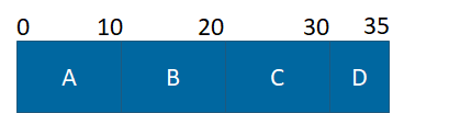
Example 1: Change Point Analysis, for a data set of 35 points where Record Count = 10 and Minimum Records = 5
All possible cost combinations are calculated:
- Cost A (0 – 10)
- Cost B (10 – 20)
- Cost AB (0 – 20)
- Cost C (20 – 30)
- Cost BC (10 – 30)
- Cost ABC (0 – 30)
- Cost ABCD (0 – 35)
- Cost BCD (10 – 35)
- Cost CD (20 – 35)
- Cost D (30 – 35)
Best segment combination is determined, for example:
- If Cost AB is less than Cost A + Cost B, then compare: AB + C vs A + BC vs ABC
- If Cost AB + Cost C is lowest, then compare: AB + C + D, vs AB + CD vs A + BCD vs ABCD (not ABC + D)
- If Cost ABC is lowest, then compare ABC + D vs ABCD vs A + BCD vs AB + CD (not AB + C + D)
- If Cost A + Cost BC is lowest, then compare: A + BCD vs A + BC + D vs AB + CD, ABCD (not ABC + D AB + C + D)
- If Cost AB is greater than Cost A + Cost B, then compare: A + B + C vs A + BC vs ABC
Usual case of changing point analysis:
To facilitate the notation, each range (x - y) will be named by their letter : A = (0 - 10), C = (20-30), BC = (10-30)..
To find the best ensemble of segment:
- The first segment to be considered will be A (0- 10)
Why not 0 to 5?
Because we have divided our data by the record count: 10, thus we can only create segment based on those letter A, B, C, D.
- We evaluate the cost of the first segment, Cost A.
- We create the next segments and evaluate the cost:
- Cost A + Cost B (the cost of A was previously calculated in 2.)
- Cost AB
- We then keep the best segments, if (Cost A + Cost B) < Cost (AB), the segments A + B are better (case (a)), (AB) otherwise (case (b))
- We can evaluate the next segments:
- Cost ABC
- Cost A + Cost BC
- In the case of (A + B) better than (AB) :
- Cost A + Cost B + Cost C
- In the case of (AB) better than (A + B):
- Cost AB + Cost C
- Like in the point 4., we keep the best segments (either: ABC, A+BC, A+B+C in the case (c), AB + C in the case (d))
- We can evaluate the last segments:
- Cost ABCD
- Cost A + Cost BCD
- Let assume the previous case (on 3.) (a) was the best:
- Cost A + Cost B + Cost CD
- Let assume the previous case (on 5.) (b) was the best:
- Cost A + Cost BC + Cost D
- By finding the best segments we have our changing points. Let assume the case (d) was the best, we have 2 changing point that occurs at 10 and 30. This leave us with 3 segment A, BC and D.
Example 2: Change Point Analysis, for a data set of 35 points where Record Count = 10 and Minimum Records = 15
What happens in a case of “minimum record” > “record count”:
To facilitate the notation, each range (x - y) will be named by their letter : A = (0 - 10), C = (20-30), BC = (10-30)..
To find the best ensemble of segment:
- As the minimum number of record is 15, The first segment to be considered will be AB (0-20)
- Why not (0 - 15)? Because we have divided our data by the record count : 10, thus we can only create segment based on those letter A, B, C, D.
- Then Why not use A as first segment ? Because we have defined our minimum record count to 15, and A is only 10 record.
- We evaluate the cost of the first segment Cost AB.
- We create the next segment, evaluate the cost and keep the best:
- Cost ABC
- /!\ not AB +C or A + BC as the segment A or C is not long enough
- We then create the last combinaison of segment, evaluate the cost and keep the best:
- Cost AB + Cost CD (the cost of AB was previously calculated in 2.)
- Cost ABCD
- /!\ not A + BCD, the segment A is not long enough. The same reason why not ABC + D, or A + B + C + D
- The algorithm will now return the best segment between (AB + CD) and ABCD. The one with the minimal cost.