Other

Script Models 

Supervised Script Model 

Create a Supervised Script Model 

The parameters for this method are defined on two tabs at the top of the page: Properties and Advanced.

On the Properties tab: 

1. Enter a Name for your model.

2. Select a Learning set from the list.

3. Select a Testing set from the list.

4. Enter a Predict variable name and an Error variable name. 

5. Select Variable Set, if required. 

6. Select variable(s) from the list for the Inputs.

7. Select a variable for the Output.

8. Click Save to generate the Model quality, Model accuracy report tabs.

On the Advanced tab: 

1. Select the script Language. Options: Javascript, R, Python and Common Lisp. 

2. Write the script. 

Script Model 

Create a Script Model 

The parameters for this method are defined on two tabs at the top of the page: Properties, Script and Advanced.

On the Properties tab: 

1. Enter script model Name. 

2. Select Variable Set, if required. 

3. Select variable(s) from the list for the Inputs.

4. Enter the Output variables of the script model. Select Type. If required, add Title and Unit. Click on +ADD to add several outputs. 

On the Script tab: 

1. Select the script Language. Options: Javascript, R, Python and Common Lisp. 

2. Write the script. 

On the Advanced tab: 

1. Select Input tasks. 

# set a value to output table 
outputTable$set(59,0L,0L) # set(numericvalue, rowindex, colindex)
outputTable$set('ABC',0L,1L) # set(symbolicvalue, rowindex, colindex)
# rem : use capital L to convert numeric to integer type

# get value by indexes
val <- inputTable$get(0L,4L) # get(rowindex, colindex)
outputTable$set(val,5L,0L)

# input table row count
rowcount <- inputTable$rowCount()
outputTable$set(rowcount,1L,0L)

# input table column count
colcount <- inputTable$colCount()
outputTable$set(colcount, 2L, 0L);

#  get column name
light = inputTable$getName(3L) # should be Light
temperature = inputTable$getName(1L) # should be Temperature
outputTable$set(light,1L,1L)
outputTable$set(temperature,2L,1L)

# find variable index by name
light_index = inputTable$findAttributeIndex('Light') # findAttributeIndex(colname); 
outputTable$set(light_index,3L,0L)  # shoud be 3

# create vector from first variable
row_count = inputTable$rowCount()
range <- 1:row_count

variable1 <- vector(length = row_count)
variable2 <- vector(length = row_count)

for (number in range){
index <- as.integer(number-1)
variable1[number] <- inputTable$get(index,0L)
variable2[number] <- inputTable$get(index,1L)
}

# compute linear regression
lr <- lm(variable2~variable1)

# get prediction
fitted <- fitted(lr)

# output linear regression
for (number in range){
index <- as.integer(number-1)
val <- fitted[number]
outputTable$set(val,index,0L)
}

Dynamic Model 

For more information, see the online learning platform

Usable for Function variables and supervised models (LR, KNN, ANN, DT, ET, MART, Adaboost, PLS, Supervised Script Model). 

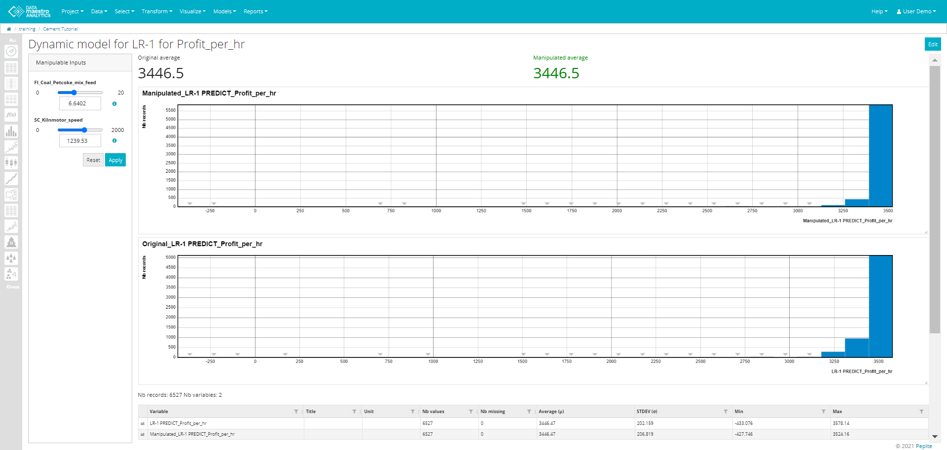
Create a Dynamic Model 

1. Enter a Title.  Note that this field is automatically filled out once the function variable/model is selected. Example: Dynamic model for Linear Regression. 

2. Enter a Manipulated variable name. Note that this field is automatically filled out once the function variable/model is selected. Example: NEW_Linear Regression. 

3. Select a Function variable / Model. 

4. Once the function or model is selected a list of Manipulable Inputs used for the function/ model appears. Select the Manipulable Inputs from the list. 

5. Select Target. Options: Maximization or Minimization. 

6. Select and Record Set, if required. 
7. Click Save. 

Partial Dependence Plots 

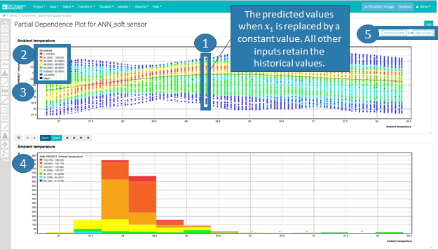
Partial Dependence Plots (PDP) are a useful visualization tool to help interpret the results of predictive machine learning models, specifically how each input influences the output variable. This tool varies each input variable one-by-one keeping all other input variables equal to historical data and calculates the new predicted values. 

1. Enter Title. 

2. Select Record Set. Define the record set to be used for calculating the predicted values. 

   Define record set

   This does not necessarily need to correspond with the Learning or Testing set used for model development, however, to avoid significant extrapolation, it is best to remain with a cleaned set of records.

3. Select Model. Currently PDPs can be calculated for all Regression supervised learning methods, with at least one numerical input.

4. Choose X Range. This is the range within which each input variable will be tested. There are two options:
   
   1. Data set min/max = The range will correspond to the min and max values for the given variable for the specified record set.
   2. 𝞵 ± N * σ = The range will correspond to Mean plus or minus N x Standard Deviation for the given variable for the specified record set.
5. Enter a Step. The number of discrete values to be tested within the X Range.
6. Select Manipulable variables. Select the variables to be manipulated. All numerical variables can be selected.

On the Advanced tab: 

1. In Scatter Plot: 

   1. Enter Conditional Class Count. For more information, see Conditional Class Count. 
   2. Select Legend Position. Options: Default and None. 
2. In Histogram: 
   1. Enter Conditional Class Count. For more information, see Conditional Class Count.
   2. Select Legend Position. Options: Default and None. 

For each manipulable variable:

1. For each step i for the given range:

a. Set the training data as the historical values and replace the historical values of 𝑥₁ with the constant 𝑥_1i.

b. Compute the predicted values for the given record set data.

c. Plot the values on the scatter plot for 𝑥₁ versus predictions.

2. The colors on the scatter plot indicate data density (or number of records).

3. The ”mean” black line, indicates the average for all predictions displayed.

4. The histogram shows the original distribution of the manipulable variable versus the model output.

5. Click Next Variable to see the results from the next selected manipulable variable.

In the example below, Ambient temperature has been varied with a step = 100. For each step, the full record set is used to compute the different predicted values for the output ANN_Soft Sensor.

Based on the scatter plot, there appears to be a parabolic relationship between ambient temperature and the output.

Looking at the histogram, however, as most data is below 30, interpretation is limited beyond this value. 

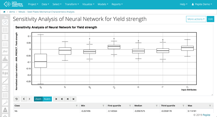
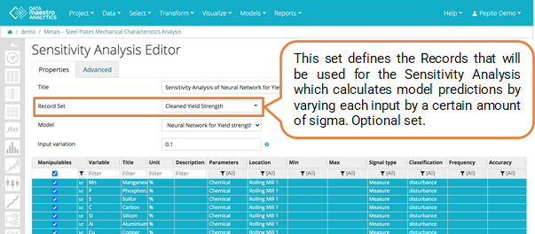
Sensitivity Analysis 

Sensitivity Analysis is a useful visualization tool to help interpret the results of predictive machine learning models, specifically how variations in each input influence the predicted output. 

Find it under Models / Other / Sensitivity Analysis.

On Properties tab: 

1. Enter Title. 

2. Select Record Set. 

3. Select a Model, all models created in the project are presented at a list. 
4. Select the Manipulable variables. 
5. Enter Input variation that is the variation applied on each input. For a Input variation equals to 0.1, each input = 0.1* 6 * sigma. 

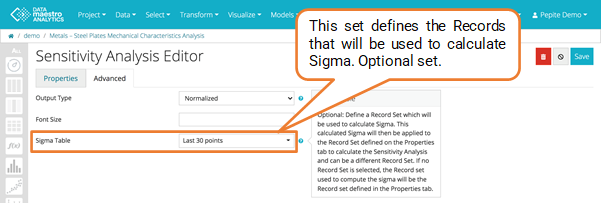
On Advanced tab: 

1. Enter Output Type. There are two types of output: 

   1. Normalized : Result = f(x + d) - f(x) / (6 * σ ) 

   2. Absolute: Result = f(x + d) - f(x)With f(x) = predicted value for one row of the dataset, f(x + d) = predicted value for one row of the dataset with an increment on one input, σ : standard deviation of predicted value on whole unmodified dataset. 

      Output Type

      By default the output variation is normalized before drawing the boxplot. In that case, all output variations are divided by six sigma of the output value in the initial datasource.  

      User can also choose to use absolute values of output variations. 
2. Enter Font Size. 
3. Select a record set in Sigma table (Optional). Define a Record Set which will be used to calculate Sigma. This calculated Sigma will then be applied to the Record Set defined on the Properties tab to calculate the Sensitivity Analysis and can be a different Record Set. If no Record Set is selectionned, the Record set used to compute the sigma will be the Record set defined in the Properties tab.

The sensitivity analysis shows how variations in each input can influence the predicted output. In the example below, the box plot shows that the output Yield Strength is influenced by the variable chemical component Niobium (Nb) followed by Nickel (Ni). 

The variables are listed in decreasing order based on the First & Third Quartile absolute values.

For example:

• If you have built a model on 12 months of cleaned data.
• Now you want to understand the influence of your different input parameters on your KPI but you want to focus your analysis on the last few days. However, over the last few days, there hasn’t been much variability in your input parameters and therefore Sigma for the last few days is low.
• At “Sigma Table” (Advance Tab), define the “Record Set” for the 12 months of cleaned data. This will calculate a sigma value, used for the Sensitivity Analysis that is representative of your full data set. This set is optional.
• Then at “Record Set” (Properties Tab), select the “Last days” set for your analysis. This set is optional.

Isolation Forest 

For more information, see the online learing platform. 

An isolation forest, is a visual representation of multiple trees used for anomaly detection. In the DATAmaestro method, data points are split randomly, with anomalies isolated in fewer steps. The depth in the tree indicates the anomaly score, with shorter paths highlighting more abnormal points and therefore potential outliers. 

For more information please refer to Wikipedia - Isolation Forest .

On Properties tab: 

1. Go to Models > Isolation Forest in the top menu. Or click the Ensemble tree icon in the left bar.

2. Enter Model name. 

3. Select at the Learning Set (Record Set). Typically, we want to use a Learning set that defines the process in the state that we want to clean. E.g. Process on and running in stable conditions.

4. Enter a Score Variable Name, Isolation forest calculates an anomaly score for each record in the Learning Set. A higher score indicates a potential outlier.
5. Select the Filter variables by.
6. Select input variables. Tip: It could be a good idea to make a Variable set to select rather than each variable individually. Search and select variable set name in the table of variables. To create a new Variable set, in Analytics, go to Select menu in top menu bar.
7. Select a Cond. one or more (Optional). E.g. product type, gauge, rate, … (Symbolic variables) For rate: calculated a symbolic version rate variable (e.g. low, medium, high rate).
8. Click Save. 

On Advanced tab: 

1. Enter a Seed. The seed for IF determines the randomness in the algorithm’s tree construction. Leave by default.

2. Enter a Tree count. Tree count in Isolation Forest specifies the number of trees in the model. Start with 100 and depending on results &/or calculation time, could be increased.

On duration curve: 

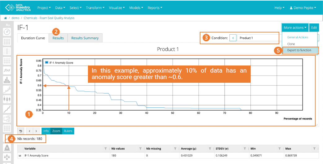
The duration curve, sorted in descending order, visualizes the anomaly scores from the Isolation Forest. Higher scores represents the most abnormal data, providing a quick overview of suspicious data for priority analysis.

1. X-axis represent the percentage of data and Yaxis represent the anomaly score.
2. Click “Result to view the anomaly score per record.
3. If any Conditions were selected, view the Duration curve per Condition. The left and right arrows change the condition.
4. See the number of associated records for the current Condition.
5. There are several options for using the Isolation score:
   1. Use the Anomaly Score directly (e.g. in Record Sets or on graphs). Caution: When updating the model, the Anomaly score will change and may no longer be a relevant value.
   2. Click on More action, Export to function” to set up a Script and keep a fixed Percentage of outliers.

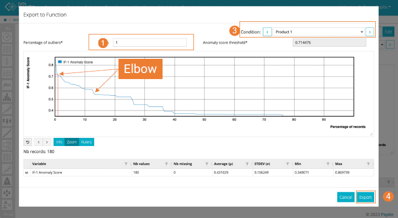
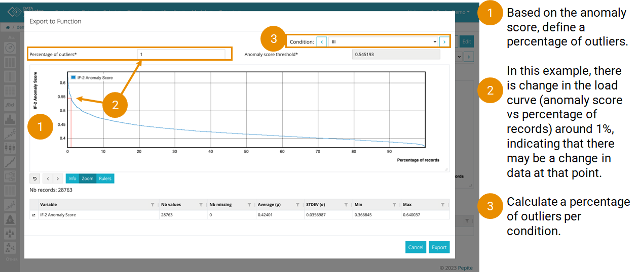
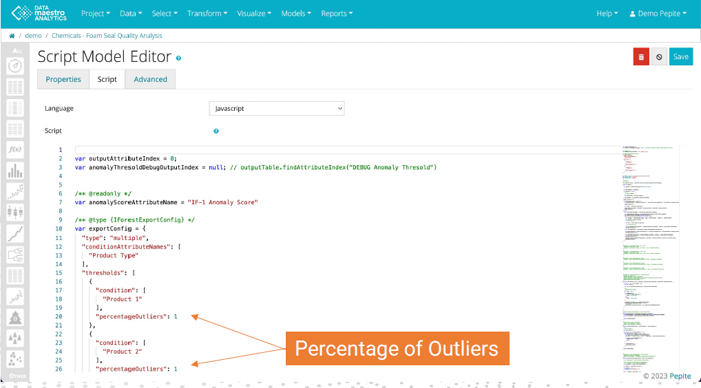
On Export to Function: 

To enhance the use of Isolation Forest, it is possible to convert the model output into a script. This facilitates the rapid selection of a specific outlier percentage and visualize of the corresponding anomaly score.

1. Enter the Percentage of outliers (for the current condition if there are multiple conditions). Next to the Percentage, the corresponding anomaly score threshold is displayed. 

   Look for an "elbow"

   Look for an “elbow” in the curve to choose a percentage of outliers. The “elbow” indicates that there is a larger difference in the points from the other closest points. Also, think about from a process view, how the process has been running and how many percentage of
   data points should be seen as outliers.

2. On the plot, the selected percentage can be visualized.
3. If a variable is conditioned, the principle remains the same; however, it is possible to choose a percentage for each condition.

On script model isolation forest: 

1. The Script Model Editor will open. Click Save. 
2. Finally the result of the script model can be used in your analysis or for data cleaning Record Sets.

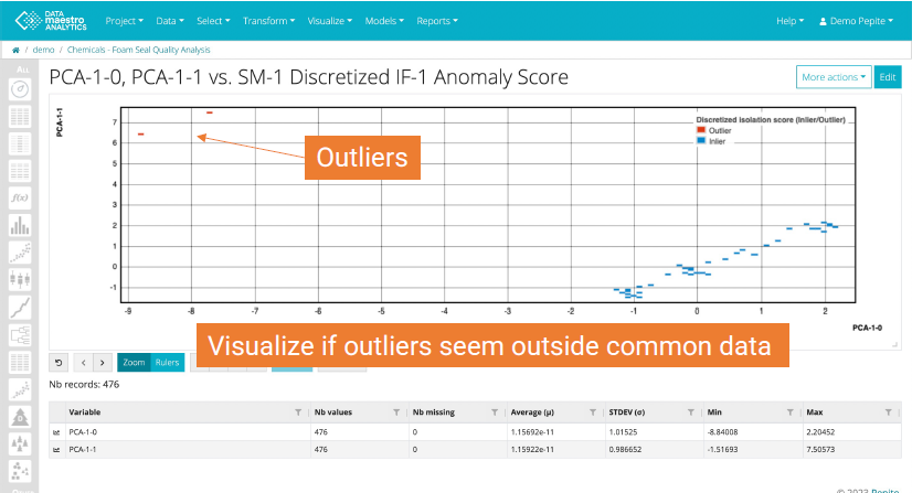
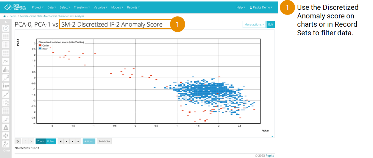
On Principal Component Analysis: 

Create a PCA to visualize the Isolation Forest results: 

1. Learning Set: Use the same Record set as for the Isolation Forest.
2. Inputs: Use the same Input Variables as for the Isolation Forest.
3. Number of components: Select 2.
4. Click Save.

Then create a scatter plot to visualize results:

1. Record set: Use the same Record set as for the Isolation Forest and PCA
2. X Axis: Select the PCA-0 variable
3. Y Axis: Select the PCA-1 variable
4. Condition: Select the SM-1 Discretized IF-1 Anomaly Score

To change Script model: 

To change the Percentage of Outliers, return to the Script Model: 

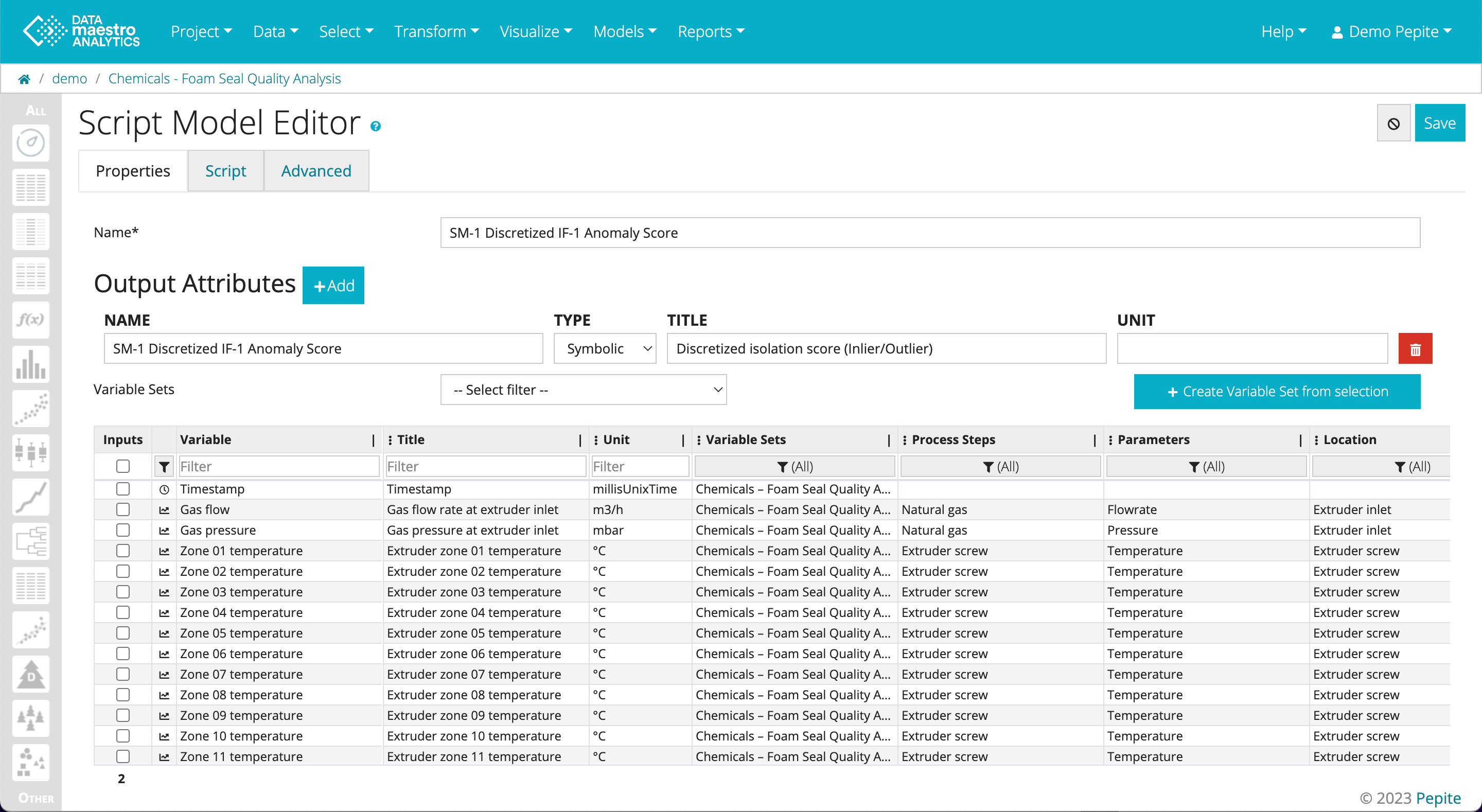
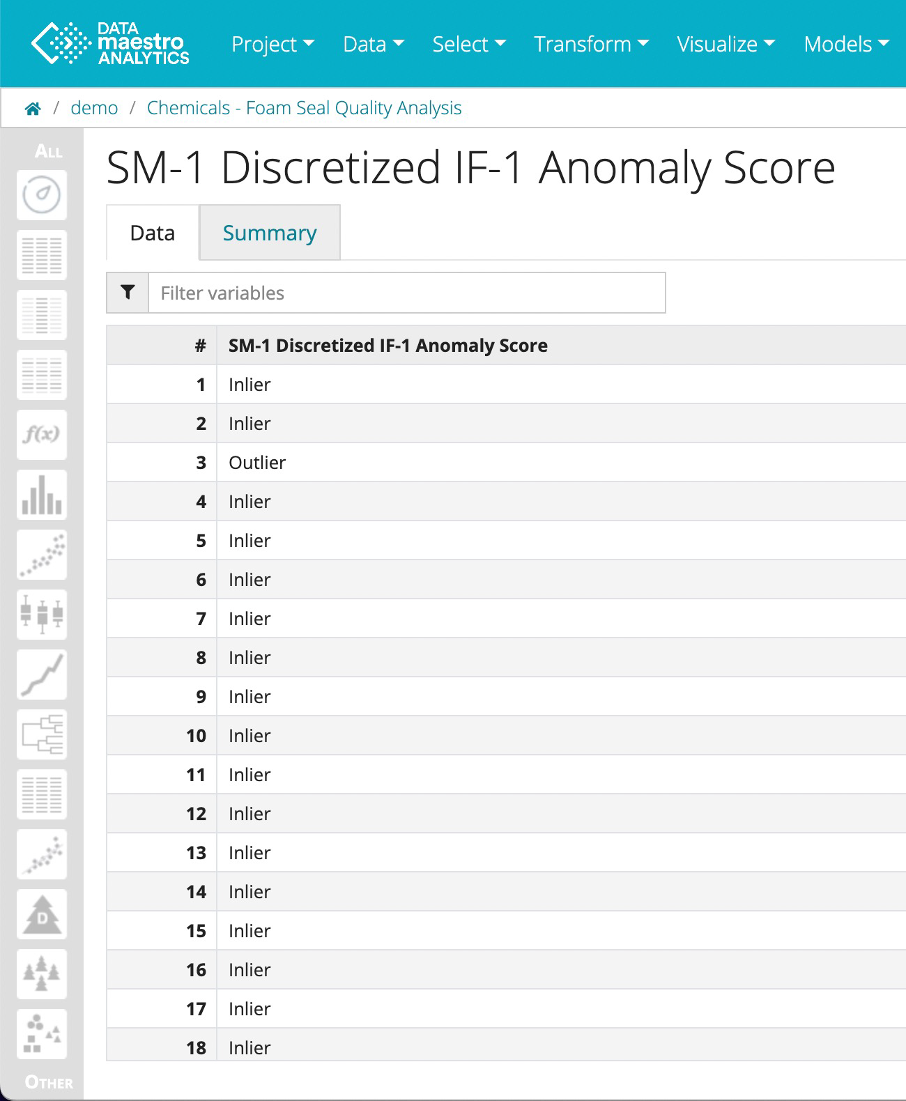
1. In the Other menu, find the SM-1 Discretized IF-1 Anomaly Score
2. Click Edit
3. Go to the Script Tab
4. Scroll down to locate the“percentageOutliers”. There will be one per condition.
5. Enter the new percentage(s)
6. Click Save

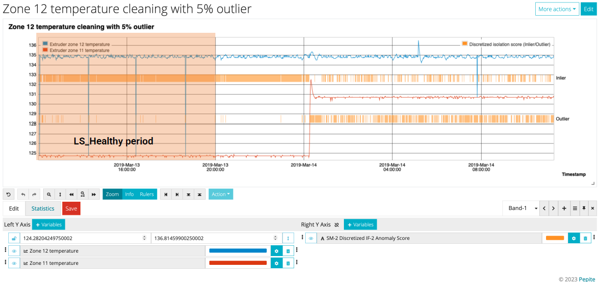
Application (5% outlier): 

• Training phase: 5% of data flagged as outliers
• Evaluation on recent data: Noticeable spike in outliers post March 14th
• Possible anomaly period detected
• Consideration: Shift in data nature or model tuning needed?
• Next steps: Manual validation, potential model updates, and further investigation of the anomaly period

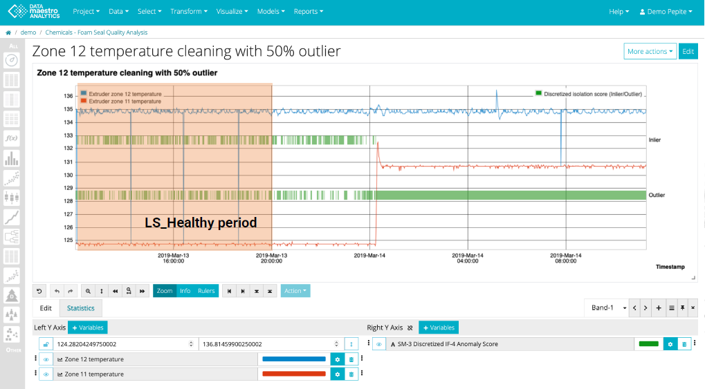
Application (50% outlier):

• New training threshold: 50% of data flagged as outliers
• Findings on recent data: Every data point post March 14th is identified as an outlier
• Implication: Significant spike in anomalies or potential model overfitting?
• Next steps: Re-evaluate threshold, manual validation, and model tuning if needed