Script Models
...
Enter a Name for your model.
Select a Learning set from the list.
Select a Testing set from the list.
Enter a Predict variable name and an Error variable name.
Select Variable Set, if required.
Select variable(s) from the list for the Inputs.
Select a variable for the Output.
Click Save to generate the Model quality, Model accuracy report tabs.
On the Advanced tab:
Select the script Language. Options: Javascript, R, Python and Common Lisp.
Write the script.
...
| Code Block | ||||||
|---|---|---|---|---|---|---|
| ||||||
# create vector from first variable
row_count = inputTable$rowCount()
range <- 1:row_count

variable1 <- vector(length = row_count)
variable2 <- vector(length = row_count)

for (number in range){
index <- as.integer(number-1)
variable1[number] <- inputTable$get(index,0L)
variable2[number] <- inputTable$get(index,1L)
}

# compute linear regression
lr <- lm(variable2~variable1)

# get prediction
fitted <- fitted(lr)

# output linear regression
for (number in range){
index <- as.integer(number-1)
val <- fitted[number]
outputTable$set(val,index,0L)
} |
For more information, see the online learning platform
Usable for Function variables and supervised models (LR, KNN, ANN, DT, ET, MART, Adaboost, PLS, Supervised Script Model).
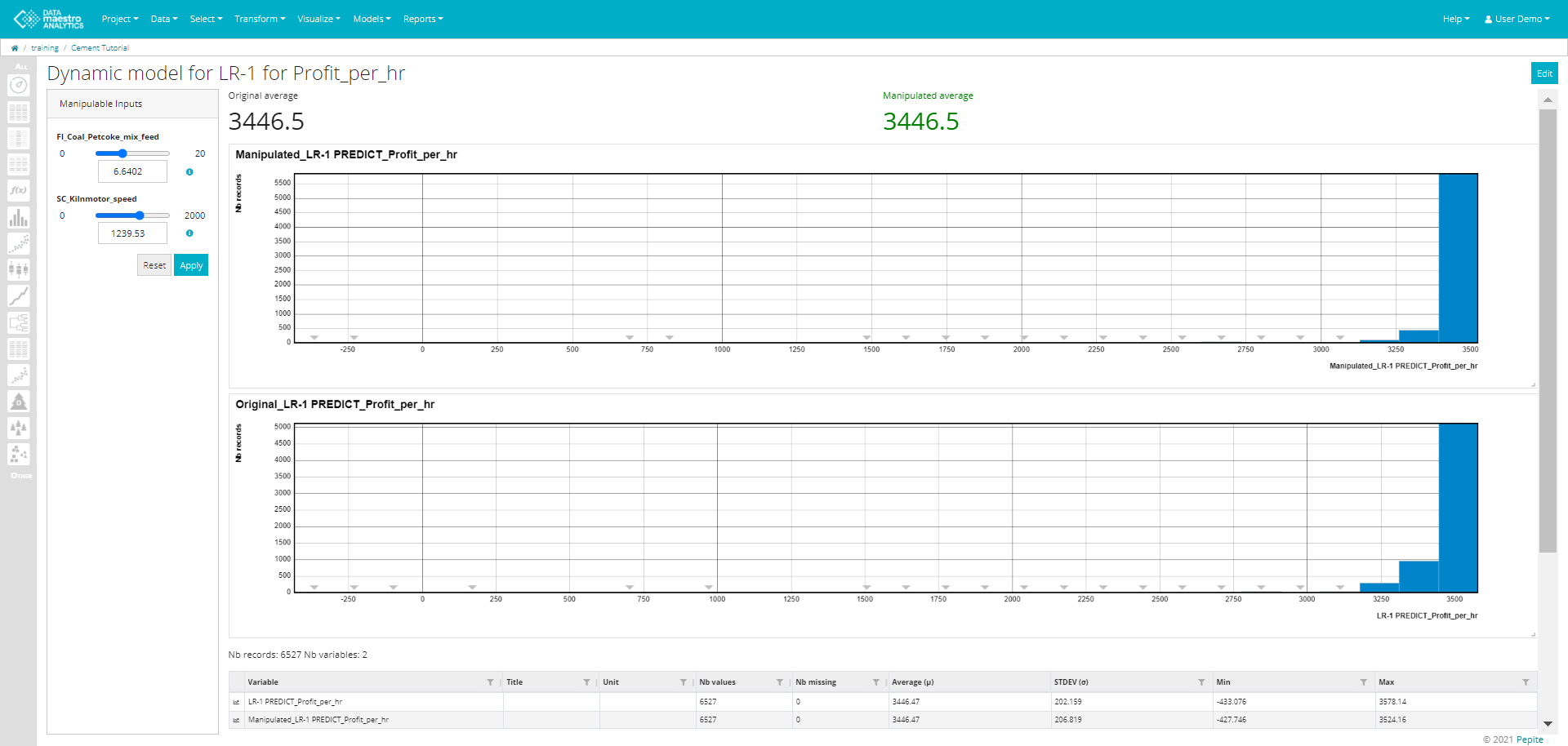
Create a Dynamic Model
- Enter a Title. Note that this field is automatically filled out once the function variable/model is selected. Example: Dynamic model for Linear Regression.
Enter a Manipulated variable name. Note that this field is automatically filled out once the function variable/model is selected. Example: NEW_Linear Regression.
Select a Function variable / Model.
Once the function or model is selected a list of Manipulable Inputs used for the function/ model appears. Select the Manipulable Inputs from the list.
Select Target. Options: Maximization or Minimization.
- Select and Record Set, if required.
- Click Save.

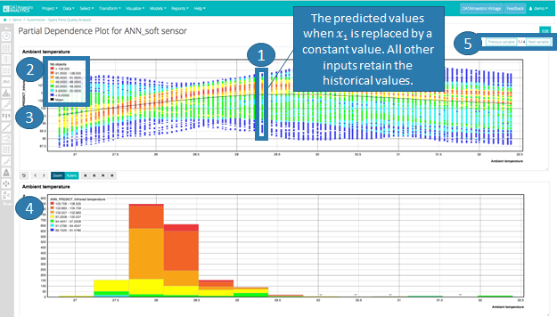
Partial Dependence Plots
Partial Dependence Plots (PDP) are a useful visualization tool to help interpret the results of predictive machine learning models, specifically how each input influences the output variable. This tool varies each input variable one-by-one keeping all other input variables equal to historical data and calculates the new predicted values.
Enter Title.
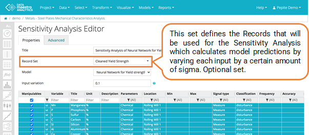
Select Record Set. Define the record set to be used for calculating the predicted values.
Info title Define record set This does not necessarily need to correspond with the Learning or Testing set used for model development, however, to avoid significant extrapolation, it is best to remain with a cleaned set of records.
Select Model. Currently PDPs can be calculated for all Regression supervised learning methods, with at least one numerical input.
- Choose X Range. This is the range within which each input variable will be tested. There are two options:
- Data set min/max = The range will correspond to the min and max values for the given variable for the specified record set.
- 𝞵 ± N * σ = The range will correspond to Mean plus or minus N x Standard Deviation for the given variable for the specified record set.
- Enter a Step. The number of discrete values to be tested within the X Range.
- Select Manipulable variables. Select the variables to be manipulated. All numerical variables can be selected.
...
Looking at the histogram, however, as most data is below 30, interpretation is limited beyond this value.

| Info | ||
|---|---|---|
| ||
If you zoom, it recalculates the steps. So if you say step = 100, then zoom on a zone, you'll have a 100 steps in that zoomed zone. |
...
Enter Title.
Select Record Set.
- Select a Model, all models created in the project are presented at a list.
- Select the Manipulable variables.
- Enter Input variation that is the variation applied on each input. For a Input variation equals to 0.1, each input = 0.1* 6 * sigma.
On Advanced tab:
Enter Output Type. There are two types of output:
Normalized : Result = f(x + d) - f(x) / (6 * σ )
Absolute: Result = f(x + d) - f(x)With f(x) = predicted value for one row of the dataset, f(x + d) = predicted value for one row of the dataset with an increment on one input, σ : standard deviation of predicted value on whole unmodified dataset.
Info title Output Type By default the output variation is normalized before drawing the boxplot. In that case, all output variations are divided by six sigma of the output value in the initial datasource.User can also choose to use absolute values of output variations.
- Enter Font Size.
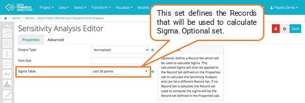
- Select a record set in Sigma table (Optional). Define a Record Set which will be used to calculate Sigma. This calculated Sigma will then be applied to the Record Set defined on the Properties tab to calculate the Sensitivity Analysis and can be a different Record Set. If no Record Set is selectionned, the Record set used to compute the sigma will be the Record set defined in the Properties tab.
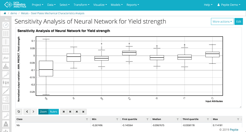
The sensitivity analysis shows how variations in each input can influence the predicted output. In the example below, the box plot shows that the output Yield Strength is influenced by the variable chemical component Niobium (Nb) followed by Nickel (Ni).
The variables are listed in decreasing order based on the First & Third Quartile absolute values.

| Info | ||
|---|---|---|
| ||
A Sensitivity Analysis can help you understand and interpret model results. For improved interpretability, define an optional Record Set for the Sigma calculation. |
...
- If you have built a model on 12 months of cleaned data.
- Now you want to understand the influence of your different input parameters on your KPI but you want to focus your analysis on the last few days. However, over the last few days, there hasn’t been much variability in your input parameters and therefore Sigma for the last few days is low.
- At “Sigma Table” (Advance Tab), define the “Record Set” for the 12 months of cleaned data. This will calculate a sigma value, used for the Sensitivity Analysis that is representative of your full data set. This set is optional.
- Then at “Record Set” (Properties Tab), select the “Last days” set for your analysis. This set is optional.


Isolation Forest
...
Go to Models > Isolation Forest in the top menu. Or click the Ensemble tree icon in the left bar.
Enter Model name.
Select at the Learning Set (Record Set). Typically, we want to use a Learning set that defines the process in the state that we want to clean. E.g. Process on and running in stable conditions.
- Enter a Score Variable Name, Isolation forest calculates an anomaly score for each record in the Learning Set. A higher score indicates a potential outlier.
- Select the Filter variables by.
- Select input variables. Tip: It could be a good idea to make a Variable set to select rather than each variable individually. Search and select variable set name in the table of variables. To create a new Variable set, in Analytics, go to Select menu in top menu bar.
- Select a Cond. one or more (Optional). E.g. product type, gauge, rate, … (Symbolic variables) For rate: calculated a symbolic version rate variable (e.g. low, medium, high rate).
- Click Save.
On Advanced tab:
Enter a Seed. The seed for IF determines the randomness in the algorithm’s tree construction. Leave by default.
- Enter a Tree count. Tree count in Isolation Forest specifies the number of trees in the model. Start with 100 and depending on results &/or calculation time, could be increased.
...
| Info | ||
|---|---|---|
| ||
|
| Info | ||
|---|---|---|
| ||
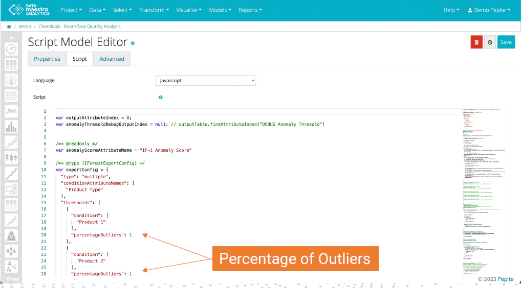
To change the Percentage of Outliers, return to the Script Model. |
To change Script model:
To change the Percentage of Outliers, return to the Script Model:
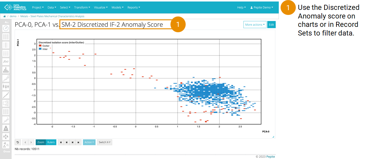
- In the Other menu, find the SM-1 Discretized IF-1 Anomaly Score
- Click Edit
- Go to the Script Tab
- Scroll down to locate the“percentageOutliers”. There will be one per condition.
- Enter the new percentage(s)
- Click Save
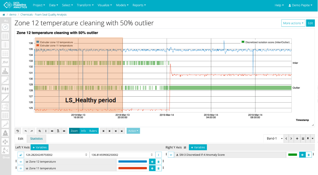
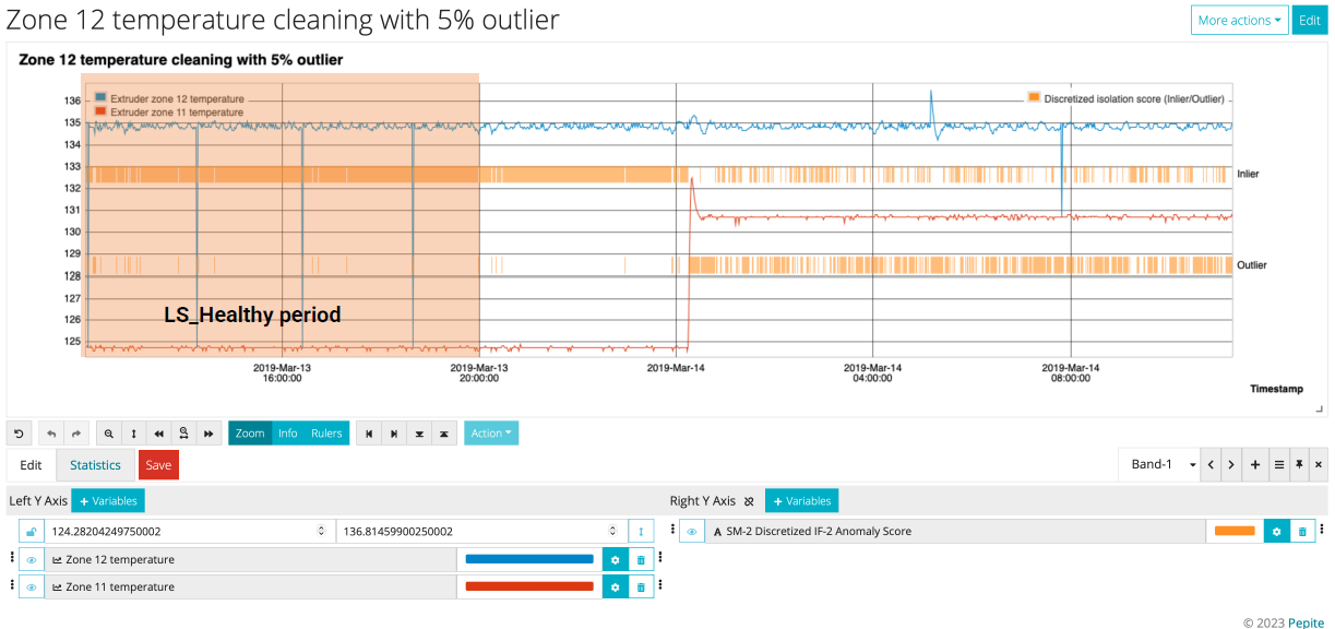
Application (5% outlier):
- Training phase: 5% of data flagged as outliers
- Evaluation on recent data: Noticeable spike in outliers post March 14th
- Possible anomaly period detected
- Consideration: Shift in data nature or model tuning needed?
- Next steps: Manual validation, potential model updates, and further investigation of the anomaly period
Application (50% outlier):
- New training threshold: 50% of data flagged as outliers
- Findings on recent data: Every data point post March 14th is identified as an outlier
- Implication: Significant spike in anomalies or potential model overfitting?
- Next steps: Re-evaluate threshold, manual validation, and model tuning if needed