About Classification Models
A classification model is a supervised learning algorithm that uses classified input variables and an output class to discover a relationship that provides an explanation or a prediction.
The inputs are numerical or categorical, and the output of the model is symbolic; it can be a level: low, high, average, or a colour: red, blue, green.
| Tip | ||
|---|---|---|
| ||
First create all the variable sets that you want to use as candidate variables in the classification model, next create all the Record sets, and then define the output classes. |
| Tip | ||
|---|---|---|
| ||
It is possible to create a new variable set using the input of the model. Click the icon |
| Tip | ||
|---|---|---|
| ||
If you want to define a color to a symbolic variable used as a Condition, use the Preferences task. For more information, check Projects. |
Decision Tree
A decision tree is a useful method for interpreting an "if then" rule structure. It is accurate for simple problems, but less accurate when the data is complex or noisy.
To launch this model tool, select Models > Decision Tree from the menu. Alternatively, click the corresponding icon in the sidebar.
| Info | ||
|---|---|---|
| ||
There is a relationship between the learning set and the number of nodes in a decision tree. By increasing the number of records for training, more information is available which allows training to develop more nodes. |
Create a Decision Tree
The parameters for this method are defined on two tabs at the top of the page: Properties and Advanced.
On the Properties tab:
Enter a Name for your model.
Select a Learning set from the list.
Select a Testing set from the list.
- Select a Datasource from the list (if applicable).
Enter a Predict variable name and an Error variable name.
Select Variable Set, if required.
Select variable(s) from the list for the Inputs.
Select a variable for the Output. In Advanced tab, check Multi Output to select more than one output.
| Tip | ||
|---|---|---|
| ||
If you don't enter an variable name for Predict or Error, the defaults are used. The suffix for these defaults includes the name of the output variable you selected. For example, "DT_PREDICT_Output" and "DT_ERROR_Output". |
8. Click Save to generate the Tree, Variable Importance, Model quality, Model accuracy report and Cross Validation (tab is deactivated if no Cross Validation strategy is used) tabs.
On the Advanced tab:
Enter a Maximum number of splits to control the branching. For more information, see Maximum number of splits.
Enter an Alpha value, usually between 0.0001 and 1.
Info title Alpha Value The closer the alpha value is to 1, the bigger the tree; 1 will develop the whole tree. Unless a pruning set is used, the results will be poor and overfit the learning set data. Typically, a value of 0.0001 provides the best results for most trees.
Check Handle missing values. For more information, see Handle missing values.
Choose a tag for Weight variable, if required. For more information, see Weight variable.
Select Pruning set. For more information, see Pruning set.
Tip title Pruning Tip Use a Pruning set to avoid overfitting. The Pruning set can be the same size as the Test set, but cannot contain records that are in the Test set or the Learning set.
- Check Enable Multi Output.
- Go to Properties tab, select the additional Outputs.
- Define Predict & Error Variable Names (Optional).
Select Cross-validation strategy, default=none. For more information, see Cross-validation.
In the example here below, we are trying to predict the power consumption level (High, Medium, Low or Very Low) with a Decision Tree model.
Here, the model was able to find that when CO2-FILLER-KG < 2606.8 and CO2-FILLER-KG<2323.7 and CO2-FILLER-KG-HL<0.445, then the power consumption level has a high probability of being "LOW" (Yellow). However, this situation doesn't happen often, according to the thickness of the condition branch ('y-y-y'). The most frequent situation is when CO2-FILLER-KG>0.2606.8, PROD-HL-BEER > 5078.09 and PROD-HL-BEER<5962.84. ('n-n-y').
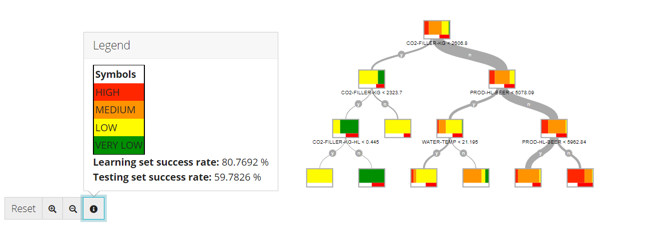
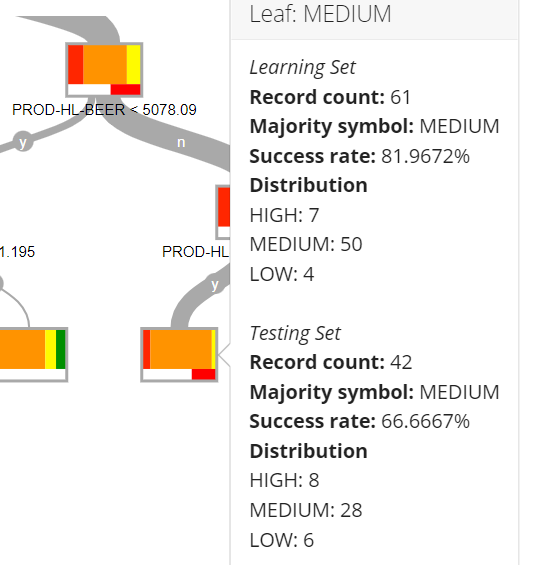
At the leaf shown here, the power is almost always "Medium" (Orange), 81.97% of time according to the Learning set. Under those condtions ('n-n-y'), the model will thus always predict "Medium". This prediction was less accurate with the testing set, as the "Medium" prediction was only correct 66.66% of the time with the testing set.
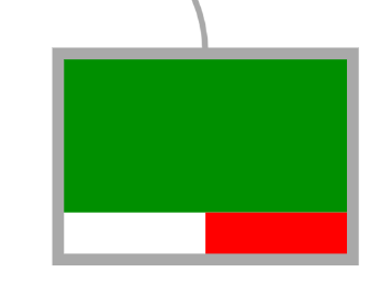
The upper and mutli-colored part of the leaf represents the population of the learning set. The white and red bar at the lower part of the leaf represents the success rate on the testing set. For example, in the square here below ('y-y-n'), it is clear that the power consumption level was always "Very Low" in the learning set, under those conditions.
However, this prediction was only accurate ~50% of the time on the testing set (50% white and 50% red).
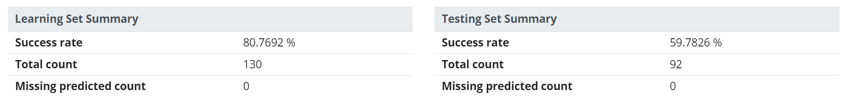
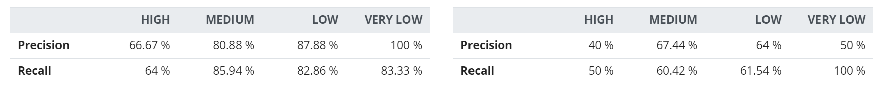
Model quality
As we saw in the previous section, if we consider the leaf ('n-n-y'), the Medium prediction of the model was correct 81.97% of the time on the Learning set, but it was correct 66.66% of the time on the testing set. That's why, the "Model Quality" shows you the overall quality on the Leaning Set and the overall quality on the Testing Set.
Quality on the Testing Set is more relevant, as it describes how your model will behave with new data. Comparing it to the quality on the Learning set is also interesting for model improvement.
 If we consider the ability of the model to predict a "High" power consumption level, the model can make several kinds of mistake:
- False Positive results: the model incorrectly predicts "High”, when it’s not High
- False Negative results: the model incorrectly predicts not "High", when it's High
On the other hand, the model can be right in two ways: - True Positive results: the model correctly predicts "High"
- True Negative results: the model correctly predicts not "High"
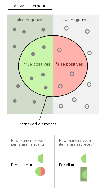
That's why it's common to use two types of metrics to evaluate the accuracy of a model: - Precision: is the ratio of True Positive amongst the elements predicted as positive (i.e. the ratio of correct predictions amongst the elements predicted as High). Precision is a metric which evaluates the ability of the model to avoid False Positive results.
- Recall: is the ratio of True Positive amongst the actual positive values (i.e. the ratio of correct predictions amongst the actual "High" elements). Recall is a metric which evaluates the ability of the model to avoid False Negative results. It is also called "sensitivity".
A dummy blind model always predicting "High" whatever the conditions will have a perfect Recall score (no false negative) but a very poor Precision score (a lot of false positive) -- example of a very sensitive model.
A dummy conservative model almost always predicting "not High" will have a very good Precision (almost no false positive), but a poor Recall score (a lot of false negative) -- example of very precise model.
Most of time, there is a trade-off between sensitivity and precision: increasing one will reduce the other one. The choice to give more importance to one or the other metric depends on the use case. Specifically, it depends on the cost of a false positive prediction and on the cost of a false negative prediction.
For example, when predicting critical failures, we may prefer to detect too many failures than taking the risk to miss some. When predicting product compliance, we may be ok to miss a few noncompliant pieces than taking the risk to throw away some compliant pieces.
The following picture can help your understanding. You can consider the actual "High" values (=actual positive values) as the full dot on the left of the square (=relevant elements)
The elements predicted as "High" (= elements predicted as positive) are the elements inside the circle.
Control the View
Use the control menu below the chart to modify the zoom and check the decision tree legend. For more information, see Control Menu.
To download data:
Click More actions and in General Actions click Download Data. A .CSV file is downloaded with data of DT_PREDICT_Output and DT_ERROR_Output.
To create a Trend:
Click More actions and in General Actions click Create Trend.
In the Trend Editor, the curve presents in Y axis the DT_PREDICT_Output and Output. The Trend is going to be displayed ONLY for Numerical outputs.
Click on Save.
To export a function:
Click More actions and in General Actions click Export to function.
Enter in the function editor a function name, if required. The suffix for this default includes the name of the output variable you selected. For example, "DT-EXPORT-Output".
Click Save.
| Info | ||
|---|---|---|
| ||
The function provided by the Decision tree is in JAVAScript format. |
Extra Trees
Ensemble trees is a robust classification model that include the most effective methods available: Bagging, Random Forest, Boosting, Mart, and Extremely Randomized Trees.
To launch this model tool, select Models > Extra trees from the menu. Alternatively, click the corresponding icon in the sidebar.
Create Extra Trees
The parameters for this method are defined on two tabs at the top of the page: Properties and Advanced.
On the Properties tab:
Enter a Name for your model.
Select a Learning set from the list.
Select a Testing set from the list.
- Select a Datasource from the list (if applicable).
Enter a Predict variable name and an Error variable name. The suffix for these defaults includes the name of the output variable you selected. For example, "ET_PREDICT_Output" and "ET_ERROR_Output".
Select variable(s) from the list for the Input.
Select a variable for the Output. In Advanced tab, check Multi Output to select more than one output.
Click Save to generate the Tree, Variable Importance, Model quality, Model accuracy report and Cross Validation (tab is deactivated if no Cross Validation strategy is used) tabs.
On the Advanced tab:
Enter an Model Count value to see the number of trees to build: between 25 and 300. For more information, see Model count.
Enter Candidate Variable Count value: between 25 and 100. For more information, see Candidate variable count.
Info title Candidate variable count There is a relationship between the learning set and the number of nodes in a decision tree. By increasing the number of records for training, more information is available which allows training to develop more nodes.
Enter a Maximum of splits to control the branching of the tree. For more information, see Maximum number of splits.
Check Handle missing values. For more information, see Handle missing values.
Enter Seed value, default value = 123456789. For more information, see Seed.
Info title Seed Seed for the randomizer. Initialization of the pseudo random series of numbers used for random part of the algorithm.
- Check Enable Multi Output.
- Go to Properties tab, select the additional Outputs.
- Define Predict & Error Variable Names (Optional).
Select Cross-validation strategy, default = none. For more information, see Cross-validation.
To download data:
Click More actions and in General Actions click Download Data. A .CSV file is downloaded with data of ET_PREDICT_Output and ET_ERROR_Output.
To create a variable set:
Click More actions and click Create variable set.
Enter the number of variables and click OK.
Enter the Variable set name, in Variable Set Editor.
Click Save.
To create a Trend:
Click More actions and in General Actions click Create Trend.
In the Trend Editor, the curve presents in Y axis the ET_PREDICT_Output and Output. The Trend is going to be displayed ONLY for Numerical outputs.
Click on Save.
Control the View
Use the control menu below the chart to modify the zoom. For more information, see Control menu.
Adaboost trees
AdaBoost is a boosting method which consists in combining an ensemble of weak models (high bias) to create a strong one.
To launch this model tool, select Models > AdaBoost trees from the menu.
Create an AdaBoost trees
The parameters for this method are defined on two tabs at the top of the page: Properties and Advanced.
On the Properties tab:
Enter a name for your model.
Select a Learning set from the list.
Select a Testing set from the list.
- Select a Datasource from the list (if applicable).
Enter a Predict variable name and an Error variable name. The suffix for these defaults includes the name of the output variable you selected. For example, "AB_PREDICT_Output" and "AB_ERROR_Output".
Select variable(s) from the list or a set of variables for the Input.
Select a variable for the Output.
Enter a Weight variable name. For more information, see Weight variable.
Click Save to generate the Tree, Variable Importance, Model quality, Model accuracy report and Cross Validation (tab is deactivated if no Cross Validation strategy is used) tabs.
On the Advanced tab:
Enter a Model count to set the number of models to be built, default= 50.
Enter a Learning rate value, to adjust the speed of convergence of the method.
Enter Maximum number of splits, it the number of splits of the trees, default = 10. For more information, see Maximum number of splits.
Check box Handle missing value, if required. For more information, see Handle missing value.
Select Loss function, options: linear, squared and exponential. For more information, see Loss function.
Enter the Weight variable, if required. For more information, see Weight variable.
Enter Seed, default=123456789. For more information, see Seed.
Select Cross-validation strategy, default = None. For more information, see Cross-validation.
To download data:
Click More actions and in General Actions click Download Data. A .CSV file is downloaded with data of AB_PREDICT_Output and AB_ERROR_Output.
To create a variable set:
Click More actions and click Create variable set.
Enter the number of variables and click OK.
Enter the Variable set name, in variable Set Editor.
Click Save.
To create a Trend:
Click More actions and in General Actions click Create Trend.
In the Trend Editor, the curve presents in Y axis the AB_PREDICT_Output and Output. The Trend is going to be displayed ONLY for Numerical outputs.
Click on Save.
Control the View
Use the control menu below the chart to modify the zoom, apply rulers to create new record sets, and to export. For more information, see Control Menu.
K-Nearest Neighbor
To launch this model tool, select Models > K-nearest neighbor from the menu.
Create K-Nearest Neighbor
The parameters for this method are defined on two tabs at the top of the page: Properties and Advanced.
On the Properties tab:
- Enter a name for your model.
- Select a Learning set from the list.
- Select a Testing set from the list.
- Select a Datasource from the list (if applicable).
- Enter a Predict variable name and an Error variable name. The suffix for these defaults includes the name of the output variable you selected. For example, "KNN_PREDICT_Output" and "KNN_ERROR_Output".
- Select variable(s) from the list or a set of variable for the Input.
- Select a variable for the Output. In Advanced tab, check Multi Output to select more than one output.
- Click Save to generate the Model quality, Model accuracy report and Cross Validation (tab is deactivated if no Cross Validation strategy is used) tabs.
On the Advanced tab:
Enter a k value, number of neighbors used by for KNN model queries, default 1. For more information, see k.
- Check Enable Multi Output.
- Go to Properties tab, select the additional Outputs.
- Define Predict & Error Variable Names (Optional).
Select Cross-validation strategy, default=none. For more information, see Cross-validation.
| Tip | ||
|---|---|---|
| ||
To visualize the KNN results use the scatter plot, choose the variables for x and y axis and then put the condition as the KNN_PREDICT_output. |
To download data:
Click More actions and in General Actions click Download Data. A .CSV file is downloaded with data of KNN_PREDICT_Output and KNN_ERROR_Output.
To create a Trend:
Click More actions and in General Actions click Create Trend.
In the Trend Editor, the curve presents in Y axis the KNN_PREDICT_Output and Output. The Trend is going to be displayed ONLY for Numerical outputs.
Click on Save.
Artificial Neural Network
To launch this model tool, select Models > Artificial neural network from the menu.
Create an Artificial Neural Network
The parameters for this method are defined on two tabs at the top of the page: Properties and Advanced.
On the properties tab:
- Enter a Name for your model.
Select a Learning set from the list.
Select a Testing set from the list.
- Select a Datasource from the list (if applicable).
Select variable(s) from the list for the Input.
Select a variable for the Output. In Advanced tab, check Multi Output to select more than one output.
Enter a Predict variable name and an Error variable name. The suffix for these defaults includes the name of the output variable you selected. For example, "ANN_PREDICT_Output" and "ANN_ERROR_Output".
Click Save to generate the Model quality, Learning Curve, Model Accuracy Report and Coefficients tabs.
On the Advanced tab:
Enter a Seed value, it initializes the random number generator used by the random part of the learning algorithm default 1234567890. For more information, see Seed.
Enter a Number of hidden layers value, is the number of additional layers to the input and output layers, not connected externally, default 1. For more information, see Number hidden layers.
Enter a Number of neurons per hidden layer value, default 20. For more information, see Number of neurons per hidden layer.
Enter a Maximum number of cycles, it limits the learning iterative process to a maximum number if no convergence is detected, default 100. For more information, see Maximum number of cycles number.
Select an Activation function from a list. For more information, see Activation function.
Select a Learning function from a list. For more information, see Learning function.
Check Skip scaling box, default false. it means the input variable are rescaled to make them numerically comparable. For more information, see Skip scaling box.
Check Skip regularization box, default false. For more information, see Skip regularization box.
Enter a Weight decay value, default 0.5. For more information, see Weight decay.
- Check Enable Multi Output.
- Go to Properties tab, select the additional Outputs.
- Define Predict & Error Variable Names (Optional).
To download data:
Click More actions and in General Actions click Download Data. A .CSV file is downloaded with data of ANN_PREDICT_Output and ANN_ERROR_Output.
To create a Trend:
Click More actions and in General Actions click Create Trend.
In the Trend Editor, the curve presents in Y axis the KNN_PREDICT_Output and Output. The Trend is going to be displayed ONLY for Numerical outputs.
Click on Save.
To export a function:
Click More actions and in General Actions click Export to function.
Enter in the function editor a function name, if required. The suffix for this default includes the name of the output variable you selected. For example, "ANN_EXPORT_Output".
Click Save.
| Info | ||
|---|---|---|
| ||
The function provided by the Artificial Neural Network is in JAVAScript format. |
To export a VBA function:
Click More actions and in General Actions click Export to VBA. Download a .TXT file with the ANN function in Visual Basic.
| Tip | ||
|---|---|---|
| ||
You can visualize the ANN (ANN_PREDICT_Output) using scatter plots and Trends. |
To clone a model:
Click More actions and click Clone as, click one of the methods in the list.
If required, edit in the model's editor.
Click Train.
| Info | ||
|---|---|---|
| ||
For the classification the clone as task can only be executed for the classification models. Therefore for example, we can't make a decision tree clone for a linear regression. |
To export a figure:
- Click More actions and click Export graphic as, choose .SVG, PDF or PNG.