Machine Automatic learning algorithms are designed to create a model of a complex system from a set of observations or simulations. The model represents relationships between the variables that describe the system. And the goal of the model is to predict the behaviour of the system in some unencountered situations or merely to explain its behaviour.

The machine learning methods described below are useful tools to solve a wide range of problems. Each method builds models in the form of new variables, which can be used as inputs for other methods. The ability to reuse models as inputs for other models gives DATAmaestro the power of hybrid approaches, where more than one learning model is used in the analysis process.

About Models

There are two main types of machine learning algorithms used to build predictive models: unsupervised and supervised.

Unsupervised Algorithms

Unsupervised algorithms are useful when you do not have a specific output variable to explain or predict. Typically, this type of algorithm is used to:

• Find a correlation or association between variables. For example, what an online shopping site would use to find baskets of goods you buy together.

• Detect clusters of records that have similar behaviour. For example, an organization of operations that are similar, like energy consumption patterns.

Supervised Algorithms

Supervised algorithms are useful when you have a value (a variable) that you want to explain (predict or model) with other variables. For example, if you want to predict the fuel consumption in your house with external temperature, air humidity, or time of the day.

To run a supervised algorithm:

1. Select a Learning set to train the model.

2. Select a Test set to test the reliability of the model.

3. Select a set of variables as inputs.

4. Identify a variable for the goal (what you try to predict with the inputs).

5. Select the type of problem (R/C/O) and the method.

6. Specify possible learning parameters for the method.

What can I do with each Supervised Learning method?

What can I do with each method?

The right technique to the right problem ! 

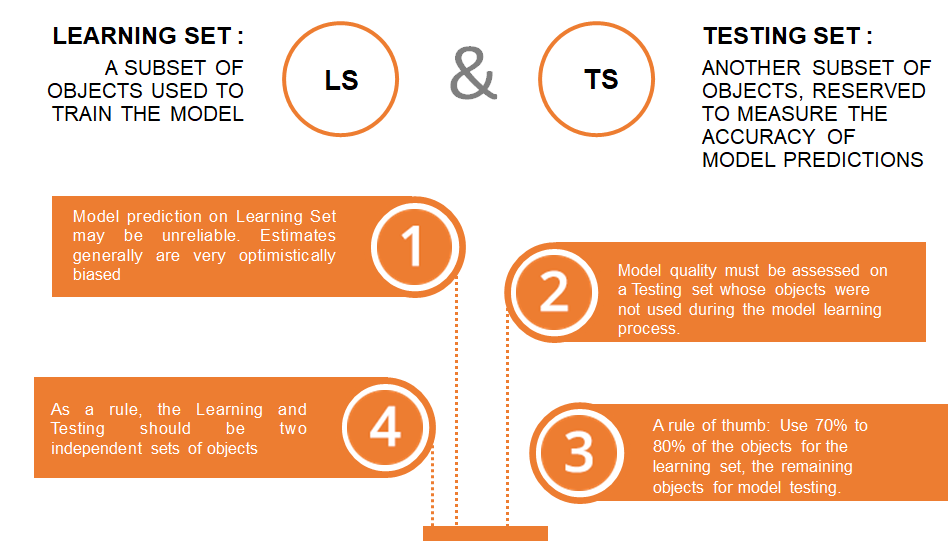
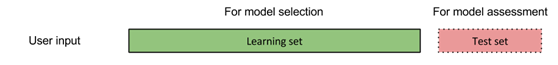
*Be careful to distinguish clustering offered by K-Means/Subclu (objective is to create clusters of similar records) from the hierarchical clustering offered by the dendrogram tool (objective is to group variables that are correlated together). In short, the first one clusters records, the second one clusters variables.

Learning and Testing sets 

Learning and Testing sets are used for supervised machine learning techniques, when the purpose is to train a model. 

1. As a rule, the Learning and Testing should be two independent sets of records.

2. The Learning set is a subset of records used to the train the model.
3. The Testing set is another subset of records used to measure the accuracy of the model predictions.
4. Typically, the Learning set is 70-80% of the total amount of records, and the Testing set records is the remaining records that are "Not In" the learning set. 

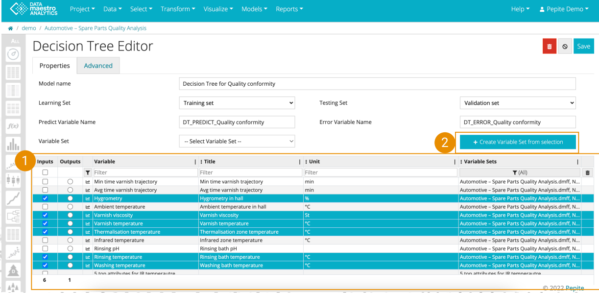
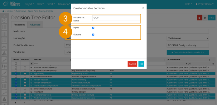
For more information, see Data.

Create Variable set

Once you have selected a list of variables, automatically create a Variable Set from the list of inputs and/outputs.

1. Select variables in the Variable picker
2. Click “Create Variable Set from selection”
3. Define a name for the Variable Set or leave by default
4. Choose whether to keep input and/or output variables and click Ok.

Multi-Output 

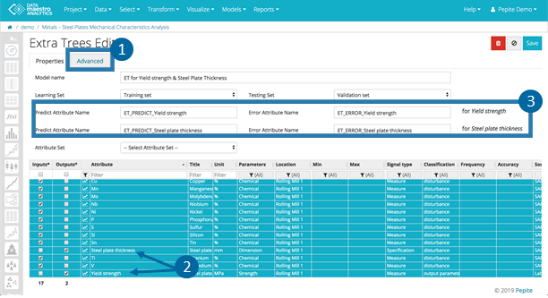
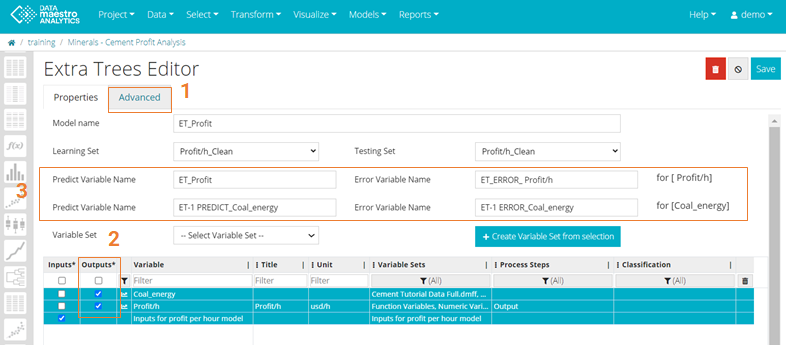
Find this option under Edit / Advanced / Enable Multi Output checkbox

1. In Advanced tab, check Enable Multi Output checkbox. 

2. Go to Properties tab and select additional outputs for the model. 

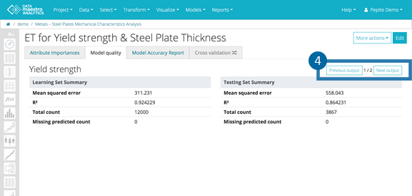
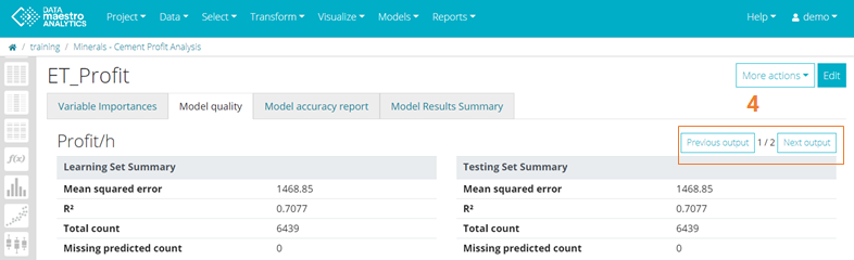
3. Define Predict and Error Variable Names, Optional.

4. Review results for model quality and accuracy. The example below illustrates an Extra Trees model, there is only one Variable Importance tab but several Model quality tabs (one for each output model). 

Cross Validation 

It is a model assessment and model selection tool. In Cross Validation, the Learning set is divided into several subsets and the model is trained on one of these subsets. Each sub-model of the Cross Validation uses the remaining partitions of the learning set as a testing set, to assess the sub-models' quality. Once the final model is created, the Testing set is used to assess the model quality and calculate the error. Several strategies for creating the partition of records are proposed: k-Fold, Stratified k-Fold, Leave-P-Label-out, Leave-P-out, Train-test split). Cross validation also helps identify the best model parameters. It is possible to enter values for the tunable parameters and the best values are presented as Cross validation results.

To launch this model tool, select in Models properties Cross validation strategy. 

Methods: 

Given a learning algorithm A and a set of parameters to evaluate, model selection is performed as follows :

• for each combination of parameters :
  • a new model is learned with the algorithm A initialized with the current set of parameters.
  • its error is evaluated on the user-provided learning set using cross-validation.
  • if the error is smaller than for all the previous models, the parameters and the model are retained as the best.
• At the end, the best model and parameters are returned and their generalization can be assessed on the test set specified by the user.

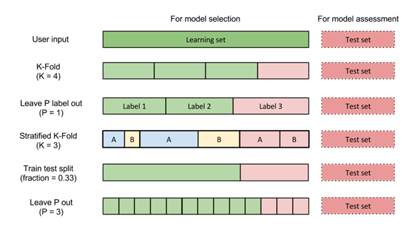
Cross-validation strategies implemented :

• KFold : explained above (see scikit learn quote)
• Stratified KFold : the various folds are built such that their output distributions are similar
• Leave-P-Out : create every possible learning set/test set combination so that P records are extracted as a test set. For each combination, a model is learned on the the N – P records and the error is evaluated on the P remaining records. The final error is the combination’s errors average (in particular, for P=1, this strategy is equivalent to the Leave-One-Out one)
• Leave-P-Label-Out : a third-party variable associates a label to each record of the dataset and is used to create the folds. Then, performs like Leave-P-Out : create every learning set/test set combination so that P groups of labels are removed. For each combination, a model is learned on the K – P groups of labels (where K is the number of distinct labels in the learning set) and the error is evaluated on the P remaining groups. The final error is the combination's errors average (in particular, for P = 1, this strategy is equivalent to leave one label out) . This strategy make sense to avoid over-fitting when some groups of records are more correlated (period of the year, people,…)
• Train/test split : same principle as for model assessment. The learning set given by the user is splitted into yet another learning set and a validation set. The model is learned on the former and evaluated on the latter. This strategy is probably the less costly (in terms of computations) but performs poorly on small datasets as “results can depend on a particular random choice for the pair of (train, validation) sets” (scikit learn user guide).

Create Cross-validation strategy

The parameters for this method are defined on tab Properties.

On the Properties tab: 

1. Select a Cross-validation strategy from the list.

2. Enter the parameters for the strategy selected.

3. Enter the values for the tunable parameters, use comma to separate the values, indicated by this icon

4. Click Train to generate the Model.

5. Check Cross-Validation tab results.

Description of Cross-validation strategies: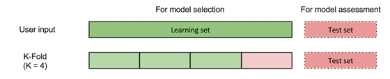 

• K-Fold: the learning set of size Nis divided in K folds of N/K records. K models are learned by taking out one different fold for each model. The error is computed by averaging the error of the model on their respective left out fold.

  • K:Number of folds, default = 3, recommended K=10.

  • Shuffle: It is a variation of the k-Fold method that can randomly shuffle data before splitting them into k folds. The parameter Seed initializes the random shuffling each time the k-Fold is iterated. Two identical seeds lead to two identical shuffling. If the box is checked, yes and no if unchecked. 

  • Seed: Initializes the random number generator used by the random part of the learning algorithm. Two identical seeds lead to two identical random number series, thus the same learning results.

• Stratified K-Fold: Same as K-Fold except that folds are computed in order to provide to each output distribution close to the overall output distribution.
  • K: Number of folders, default = 3, recommended K = 10.
  • Output variable:Select the variable from the list. 
  • Seed:Initializes the random number generator used by the random part of the learning algorithm. Two identical seeds lead to two identical random number series, thus the same learning results.

• Label-P-Label-Out: Create folds based on third-party symbol variable, a given fold contains all records associated with a given label. This label can be period of the year or a record.
  • P: Number of folds, default = 1. 
  • Label variable: Select  the variable containing the label.

• Leave-P-out: The folds are created so that every combination of P records are removed. This method is useful for small data set but very expensive for large ones.
  • P = Number of folds, default = 1. 

 Description: 

For Leave-P-out the time of resolution of an algorithm is dependent on the number of records in the training set.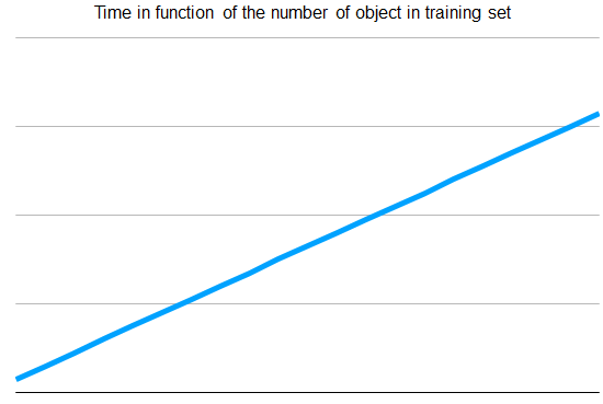 

       The number of records in the training set is inversely proportional to P. If the data set has 300 records and if P=50.

Training set has 250 records. The result is as P increase, the time to train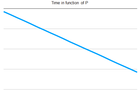

       The number of algorithms to be tested is dependent of the number P with a binomial distribution. 

       The addition of these two effects leads that a small value of P will lead to a slower Cross-validation.

• Train-Test split: It splits the learning set into training set and validation set. This method uses only one model to assess the error of a combination of parameters. It is the fastest method.
  • Test fraction (%): Split fraction used by the Train/Test split strategy cross-validation. It defines the fraction of records that should be extracted from the learning set where the remaining records make up the validation set.
  • Seed: Initializes the random number generator used by the random part of the learning algorithm. Two identical seeds lead to two identical random number series, thus the same learning results.

モデル

自動機械学習アルゴリズムは、観測値哉シミュレーションのセットから複雑なシステムのモデルを作成するように設計されています。モデルはシステムを説明する変数の間の関係を表します。モデルの目標は、発生していない状況やほとんど発生しない状況でのシステムの動作を予測し、その動作を説明することです。

次に説明する機械学習方法は、さまざまな問題を解決するのに役立つツールです。各方法では、他の方法の入力として使用できる新しい属性という形式でモデルを構築します。DATAmaestro では、モデルを他のモデルの入力として再利用できるため、ハイブリッドアプローチによって複数の学習モデルを分析プロセスで使用できます。

モデルについて

予測モデルを構築するために使用される機械学習アルゴリズムには、主に「教師なし」と「教師あり」という 2 種類があります。

教師なしアルゴリズム

説明または予測する特定の出力変数がないときには、教師なしアルゴリズムが役立ちます。一般的に、このタイプのアルゴリズムは次の目的で使用されます。

• 属性間の相関関係または関連付けを見つける。たとえば、オンラインショッピングサイトでまとめて購入する商品を見つけるために使用するアルゴリズムです。
• 類似した動作のオブジェクトのクラスターを検出する。たとえば、エネルギー消費パターンなどの類似した事業の組織です。

教師ありアルゴリズム

他の属性で説明 (予測またはモデル化) する値 (属性) があるときには、教師ありアルゴリズムが役立ちます。たとえば、屋外の気温、空気湿度、日照時間を使用して住宅の燃料消費量を予測する場合です。

教師ありアルゴリズムを実行する

1. モデルを学習する学習セットを選択します。
2. モデルの信頼性をテストするテストセットを選択します。
3. 入力として属性のセットを選択します。
4. 目標の属性を特定します (入力を使用して予測しようとする属性)。
5. 問題の種類 (R/C/O) と方法を選択します。
6. その方法で考えられる学習パラメーターを指定します。

必要な学習セットとテストセット

学習モデルを構築する前に、学習とテストにそれぞれ 1 つずつ、合計 2 つのオブジェクトセットを用意する必要があります。

問題に適した手法が必要です。 

学習セットとテストセット 

モデルを学習するときには、教師あり機械学習手法で学習セットとテストセットが使用されます。原則として、学習とテストは 2 つの独立したオブジェクトのセットです。学習セットはモデルの学習で使用されるオブジェクトのサブセットです。テストセットはモデルの予測の精度を測定するために使用されるオブジェクトの別のセットです。一般的に、学習セットは合計オブジェクト数の 70～80% です。テストセットオブジェクトは学習セットには含まれていない残りのオブジェクトです。

詳細については、データを参照してください。

複数出力 

モデルの複数出力 

同じ入力に基づいて、複数出力変数で 1 つの教師あり予測モデルを学習します。 

次のアルゴリズムで使用できます。線形回帰、決定木、Extra Trees、k近傍法、人工ニュートラルネットワーク

[編集] / [詳細] / [複数出力を有効にする] チェックボックスの下でこのオプションを見つけます。

1. [詳細] タブで [複数出力を有効にする] チェックボックスをオンにします。 
2. [プロパティ] タブに移動し、モデルの追加出力を選択します。 
3. 予測およびエラー属性名を定義します (任意)。
4. 結果でモデルの品質と正確性を確認します。次の例の図は Extra Trees モデルです。[属性重要度] タブは 1 つだけですが、複数の [モデル品質] タブ (出力モデルごとに 1 つ) があります。 

交差検証 

交差検索はモデル選択で使用できます。特定の学習アルゴリスムとパラメーターセットで、エラーが評価されます。

このモデルツールを起動するには、[モデル] プロパティで [交差検証手法] を選択します。 

方法: 

機械学習アルゴリズム A と評価するパラメーターセットが与えられた場合、次のようにモデル選択が実行されます。

• パラメーターの各組み合わせ: 
• 新しいモデルは、現在のパラメーターセットで初期化されたアルゴリズム A で学習されます。
• 交差検証を使用して、ユーザーが指定した学習セットでエラーが評価されます。
• エラーがすべての前のモデルよりも小さい場合、パラメーターとモデルは最適であるため維持されます。
• 最後に、最適なモデルとパラメーターが返されます。ユーザーが指定したテストセットで汎化を評価できます。

導入された交差検証手法:

• KFold (k分割) : 上記の説明を参照 (scikit 学習ガイドを参照)
• Stratified KFold (階層化 k分割) : 出力の分布が類似するようにさまざまな分割が構築されます。
• Leave-P-Out : P オブジェクトがテストセットとして抽出されるように、すべての考えられる学習セット/テストセットの組み合わせを作成します。各組み合わせでは、モデルが N – P オブジェクトで学習され、P 残りオブジェクトでエラーが評価されます。最終的なエラーはその組み合わせのエラー平均です (特に、P=1 の場合、この手法は Leave-One-Out と同じになります)。
• Leave-P-Label-Out (リーブ P ラベルアウト): サードパーティ属性がラベルをデータセットの各オブジェクトに関連付け、分割を作成するために使用されます。次に、Leave-P-Out などを実行します。ラベルの P グループが削除されるように、すべての学習セット/テストセットの組み合わせを作成します。各組み合わせでは、ラベルの K - P グループでモデルが学習されます (K は学習セットの一意のラベル数)。エラーは P 残りグループで評価されます。最終的なエラーはその組み合わせのエラー平均です (特に、P=1 の場合、この手法は Leave-One-Label-Out と同じになります)。一部のオブジェクトのグループの相関関係が強い (年の期間、人など) ときに過学習を回避するには、この手法が有効です。
• 学習/テストの分割 : モデル評価と同じ原理。ユーザーが指定した学習セットは別の学習セットと検証セットに分割されます。モデルは学習セットで学習され、検証セットで評価されます。この手法は (演算という点で) コストが低いと考えられますが、「結果が (学習、検証) セットの組み合わせの特定のランダム選択に依存することがある」ため、小さいデータセットでは良い結果が得られません (scikit  学習ユーザーガイド)。

交差検証手法の作成 

この方法のパラメーターは [プロパティ] タブで定義されます。

[プロパティ] タブ: 

1. リストから交差検証手法を選択します。
2. 選択した手法のパラメーターを入力します。
3. 調整可能なパラメーターの値を入力し、カンマを使用してこのアイコンが表示されている値を区切ります。
4. [学習] をクリックして、モデルを生成します。
5. [交差検証の確認] タブに結果が表示されます。

交差検証手法の説明 

• K分割: サイズ N の学習セットが N/K オブジェクトの K 分割に分割されます。K モデルは各モデルで 1 つの異なる分割を取り出して学習されます。それぞれの残された分割でモデルのエラーを平均化して、エラーが計算されます。
• K = 分割数。既定値 = 3、推奨値 K=10
• シャッフル = チェックボックス。[はい] または [いいえ]。既定値= いいえ。データをシャッフルして独立したフォルダーを作成。

• 階層化K 分割: K 分割と同じ。ただし、全体的な出力分布に近い各出力分布を生成するために分割が計算されます。 
• K = 分割数。既定値 = 3、推奨値 K=10
• シャッフル = チェックボックス。[はい] または [いいえ]。既定値= いいえ。データをシャッフルして独立したフォルダーを作成。
• 出力属性 = 出力属性 

• Label-P-Label-Out: サードパーティ記号属性に基づいて分割を作成します。特定の分割には、特定のラベルに関連付けられたすべてのオブジェクトが含まれます。このラベルは年の期間またはオブジェクトにすることができます。 
• P = 分割数。既定値 = 1 
• ラベル属性 = ラベルを含む属性。     

• Leave-P-out: P オブジェクトのすべての組み合わせが削除されるように分割が作成されます。このモデルは小さいデータセットは有効ですが、大きいデータセットでは非常にコストが高くなります。 
• P = 分割数。既定値 = 1 
• ラベル属性 = ラベルを含む属性。 

説明: 

Leave-P-out では、アルゴリズムの解決時間が学習セットのオブジェクト数に依存します。 

       学習セットのオブジェクト数は P に反比例します。データセットのオブジェクトが 300 で P=50 の場合、

学習セットのオブジェクトは 250 です。P が増えると、学習時間が増えます。

       テストされるアルゴリズム数は2項分布で P の数に依存します。 

       これらの 2 つの効果が追加され、小さい値の P の交差検証は低速になります。

警告

交差検証モデルの品質は学習セットのオブジェクト数に関連付けられます。

P の値を大きくしすぎると高速になりますが、使用に適さないモデルになります。

• 学習/テストの分割: 学習セットを、学習セットと検証セットに分割します。この方法は 1 つのモデルのみを使用して、パラメーターの組み合わせのエラーを評価します。最速の方法です。

• 割合のテスト: 学習セットから抽出されるオブジェクトの割合。既定値 = 0.33